Under the bonnet
If you’re interested in how this script works, or would like modifications, here I’ll describe how it works.
What is going on?
preprocess.py is simply an elaborate way of calling the SNAP graph processing tool (gpt) with pre-determined processing chains. The Python element deals with different input data (ALOS-1/ALOS-2 data), and automates the creation of new file names. The processing chains are stored in the approach/cfg/ directory, and these are used by the Python script by specifying the flags -Pinputfile and --Poutputfile. For example, to process an ALOS-1 file the Python script may submit the command:
~/snap/bin/gpt approach/cfg/SNAP_chain_A1.xml -x -Pinputfile=~/ALOS_data/ALPSRP076546990-L1.1.zip -Poutputfile=ALOS1_HV_20070702_ALPSRP076546990.tif
and to process an ALOS-2 file the Python script you would submit:
~/snap/bin/gpt approach/cfg/SNAP_chain_A2.xml -x -Pinputfile=~/ALOS_data/0000149017_001001_ALOS2117217000-160724.zip -Poutputfile=ALOS2_HV_20160724_ALOS2117217002-160724.tif
If you want to use a different pre-processing chain, the place to begin would be to modify the files approach/cfg/*.xml using the SNAP Graph Builder. I can recommend a look through the SNAP forum to get a better idea of how the graph processing tool works.
mosaic.py is a set of commands to assist in the automation of generating mosaic products. The script relies heavily on GDAL/OGR to reproject images to a single output CRS, and uses numpy to generate a mean output image.
What is the processing chain for ALOS-1?
The processing chain for ALOS-1 looks like this:
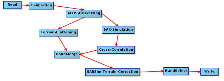
The steps are:
- Calibration: Radiometrically corrects the SAR image so that pixel values represent the radar backscatter of the reflecting surface.
- ALOS deskewing: Required only for ALOS-1 data, as the data is distributed in a squinted geometry. Deskewing transfers the data into a zero Doppler geometry, which is necessary before applying standard SAR processing.
- Terrain-Flattening: This step improves radiometric calibration by removing topographic effects. This will, for example, correct for the tendency for surfaces that area angled towards the sensor to be recorded as brighter.
- SAR-Simulation: This step simulates the image that would be expected given topographic effects alone.
- Cross-Correlation: The recorded backscastter is correlated with that expected from topography. Step 4 must be conducted in parallel with step 3, as radiometric terrain flattening removes the very terrain features that SARSim requires to align images to the DEM.
- BandMerge: Images from steps 3 and 4/5 are added to a single image.
- SARSim-Terrain-Correction: Terrain Correction will geocode the image by correcting SAR geometric distortions using a DEM and producing a map projected product. We use SARSim TC as the geometric accuracy when using Range-Doppler TC (which uses dead reckoning) is otherwise poor. SARSim TC warps the image to the expected topographic features. It may not work well given very flat topography.
- BandSelect: Selects the band to output.
- Write: Writes output to a geotiff file.
What is the processing chain for ALOS-2?
The processing chain for ALOS-2 looks like this:
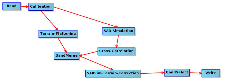
The processing chain we have selected for ALOS-2 is identical to ALOS-1, but omits the ALOS-deskewing step which is not required for ALOS-2.
We still perfrosm SARSim terrain correction, though note that Range Dopper terrain correction is probably more appropriate for ALOS-2 with its better geolocation accuracy. The reason we still use SARSim terrain correction is so that the outputs better match those of ALOS-1. If we compare the outputs of Range Doppler TC for ALOS-2 and SARSim TC for ALOS-1, we find that shifts between the two images are much greater than if we accept the additional error and processing time introduced by SARSim TC.
What about speckle filtering?
Speckle filtering is handled by two additional .xml files (SNAP_chain_filter_A1.xml/SNAP_chain_filter_A2.xml). These insert a lee-filter operator before the terrain flattening step. In some cases this can dramatically increase the processing time, for reasons that aren’t clear yet.
How can this be improved?
This is by no means the perfect solution. A more complete processing chain for pre-processing ALOS-1 and ALOS-2 data might:
- Include an additional step to warp images to a reference image to improve comparability.
- Include a method to cross-calibrate backscatter from ALOS-1 and ALOS-2, which are at present do not appear to be calibrated identically (histogram matching?).
- Do something about the profusion of error messages from SNAP and snappy :/.
What other options do I have?
ALOS data can also be processed using ASF MapReady (no longer updated) or GAMMA (commercial). Both are probably more straightforward than this approach, but this script is free and (at the time of writing, Jan 2018) up-to-date.
A pre-processed ALOS mosaic product is made freely available from JAXA, and geolocation accuracy is excellent. However you will have to accept that the dates imagery come from are not always ideal, and that you cannot take the average of multiple images to reduce the impacts of speckle.
If you are interested in using the ALOS mosaic product, we’ve also built a Python module to assist in the ingestion and processing of this data. Its available at: